# Data transformation II
```{r}
#| include: false
# settings, placed in a chunk that will not show in the .html file (because include=FALSE)
# disables scientific notation so that small numbers appear as eg "0.00001" rather than "1e-05"
options(scipen = 999)
```
This chapter continues with "*non-aggregating*" functions, i.e., functions that do not reduce many rows down to fewer summary rows. It covers changing the order of rows with `arrange()`, keeping rows based on their position with the `slice_()` functions, dropping rows with missing values with `drop_na()`, and a set of more advanced ways of using `mutate()`: handling missing values, modifying many columns at once, calculating scores across columns, using values from other rows, and filling in empty cells.
## `arrange()` and `desc()`
Arrange (`arrange()`) and descending (`desc()`) allow you to change the order of the rows without changing their contents. `desc()` is almost always used inside `arrange()`, i.e., `arrange(desc(variable))`.
```{r}
#| include: false
# generate some messy demographics data with a larger N
# devtools::install_github("ianhussey/truffle")
library(truffle)
library(dplyr)
set.seed(42)
dat_demographics_messy <- data.frame(id = 1:500) %>%
truffle::truffle_demographics() %>%
truffle::dirt_demographics()
```
```{r}
library(dplyr)
library(tidyr)
library(readr)
library(stringr)
library(knitr)
library(kableExtra)

dat_gender_tidier_counts <- dat_demographics_messy %>%
  # convert to lower case and remove non-letters
  mutate(gender = str_to_lower(gender),
         gender = str_remove_all(gender, "[^A-Za-z]")) %>%
  # tidy up cases
  mutate(gender = if_else(condition = gender %in% c("female", "male", "nonbinary"), # the logical test applied: is 'gender' one of the following
                          true = gender, # what to do if the test is passed: keep the original gender response
                          false = NA_character_))  %>% # what to do if the test is failed: set it to NA
  # count frequencies of each unique value in the gender column
  count(gender)

# arrange by increasing N
dat_gender_tidier_counts %>%
  arrange(n) %>%
  kable() %>%
  kable_classic(full_width = FALSE)
# arrange by decreasing N
dat_gender_tidier_counts %>%
  arrange(desc(n)) %>%
  kable() %>%
  kable_classic(full_width = FALSE)
# arrange by gender in alphabetical order
dat_gender_tidier_counts %>%
  arrange(gender) %>%
  kable() %>%
  kable_classic(full_width = FALSE)
# arrange by gender in reverse alphabetical order
dat_gender_tidier_counts %>%
  arrange(desc(gender)) %>%
  kable() %>%
  kable_classic(full_width = FALSE)
```
Notice that the `NA` row is placed last whether you use `arrange(gender)` or `arrange(desc(gender))`. `arrange()` always puts missing values at the end.
Note that you can also arrange by multiple columns, e.g., `dat %>% arrange(timepoint, condition, gender)` would arrange timepoint in ascending order (1, 2), then for ties it arranges condition alphabetically ("control", "intervention"), and for ties it would arrange gender alphabetically (e.g., "female", "male", "non-binary").
#### Exercise
Using the 'dat_demographics_messy' data frame, write code to arrange participants from oldest to youngest, and for participants with the same age, by their id in ascending order. Print only the first 10 rows using `head(10)`.
Hint: what type of data is the 'age' column? Check with `class()` or `glimpse()`, and use what you learned in the previous chapter to deal with it.
```{r}
#| include: false
```
::: {.callout-note collapse="true" title="Click to show answer"}
```{r}
dat_demographics_messy %>%
  # 'age' contains non-numbers, so it is a character column.
  # Arranging characters is done alphabetically, so "9" would come before "80".
  # Remove non-numbers and convert to numeric first.
  mutate(age = str_remove_all(age, "[^0-9\\.]"),
         age = as.numeric(age)) %>%
  arrange(desc(age), id) %>%
  head(10) %>%
  kable() %>%
  kable_classic(full_width = FALSE)
```
Note that arranging a character column that contains numbers sorts it alphabetically, not numerically: "100" comes before "25", which comes before "9". Always check the type of the column you are arranging.
:::
## `filter()` derivatives
Sometimes we want to `filter()` for rows not based on their content but their location, eg at the top or the bottom of the data frame. These `filter()` derivatives are therefore related to `arrange()` in that they often relate to row number rather than row contents.
### `slice_()` functions
- `slice_head(n = 5)` is equivalent to `filter(row_number() <= 5)`
- `slice_tail(n = 5)` is equivalent to `filter(row_number() > n() - 5)`
- `slice_min(x, n = 5)` is equivalent to `filter(min_rank(x) <= 5)`
- `slice_max(x, n = 5)` is equivalent to `filter(min_rank(desc(x)) <= 5)`
```{r}
# the three most common gender responses
dat_gender_tidier_counts %>%
  slice_max(n, n = 3) %>%
  kable() %>%
  kable_classic(full_width = FALSE)
```
Note that the column used by `slice_min()` and `slice_max()` (here, the column named 'n') is a different thing to the argument `n =` (the number of rows to return). It's unfortunate that the column that `count()` creates and this argument share the same name.
Also note that, by default, `slice_min()` and `slice_max()` keep ties. If two rows are tied for third place, you will get four rows back, not three. You can change this with `with_ties = FALSE`, but then which of the tied rows is dropped is essentially arbitrary.
Sometimes you might want to filter rows randomly rather than at the top or bottom of the data frame. You can do this with `slice_sample()`:
- `slice_sample(n = 5)` : return 5 random rows
- `slice_sample(prop = .05)` : return a random 5% of the rows
Because the rows are chosen randomly, you will get different rows each time you run the code. To make it reproducible, set the seed of the random number generator first with `set.seed()`:
```{r}
set.seed(42)

dat_demographics_messy %>%
  slice_sample(n = 5) %>%
  kable() %>%
  kable_classic(full_width = FALSE)
```
#### Exercise
Write code to return the rows of the three youngest participants in 'dat_demographics_messy'. Make sure that 'age' is numeric first. How many rows are returned? Why?
```{r}
#| include: false
```
::: {.callout-note collapse="true" title="Click to show answer"}
```{r}
dat_demographics_messy %>%
  mutate(age = str_remove_all(age, "[^0-9\\.]"),
         age = as.numeric(age)) %>%
  slice_min(age, n = 3) %>%
  kable() %>%
  kable_classic(full_width = FALSE)
```
Many more than three rows are returned, because of ties: lots of participants share the youngest age, 18. If you really need exactly three rows, you can add `with_ties = FALSE`, but think about whether it makes sense to arbitrarily choose three of the 18-year-olds.
:::
### `drop_na()`
A common negative-`filter()` is to remove rows whose values are `NA`. Because `NA` is a special value, this is not done with `filter(variable != NA)` but instead with its own function: `is.na()`:
```{r}
dat_gender_tidier_counts %>%
  # arrange by decreasing N
  arrange(desc(n)) %>%
  # negative filter rows where gender is not NA
  filter(!is.na(gender)) %>%
  kable() %>%
  kable_classic(full_width = FALSE)
```
This negative filter is so common that it has its own helper function: `drop_na()`, from the {tidyr} package. Note that there is also a base-R `na.omit()`, which you should avoid because it always applies to all columns.
You can pass one, more than one, or no column names to `drop_na()`. If no column names are specified, it requires that all columns are not `NA`. For example:
```{r}
# retain all rows
dat_gender_tidier_counts %>%
  kable() %>%
  kable_classic(full_width = FALSE)
# drop NA rows in 'gender'
dat_gender_tidier_counts %>%
  # negative filter rows where !is.na(gender)
  drop_na(gender) %>%
  kable() %>%
  kable_classic(full_width = FALSE)
# drop NA rows in 'gender' and 'n'
dat_gender_tidier_counts %>%
  # negative filter rows where !is.na(gender) & !is.na(n)
  drop_na(gender, n) %>%
  kable() %>%
  kable_classic(full_width = FALSE)
# drop NA rows in all columns in data frame
dat_gender_tidier_counts %>%
  # negative filter rows where all columns are not NA
  drop_na() %>%      # <- note no columns supplied to drop_na()
  kable() %>%
  kable_classic(full_width = FALSE)
```
`drop_na()` with no columns specified is convenient but risky: in a data frame with many columns, a participant can be dropped because of a missing value in a column you don't care about. As with `select()` and `filter()`, it is usually better to be explicit and name the columns.
## Missing data codes: `na_if()`
The rest of this chapter uses a small made-up survey data set. Each row is a participant. Missing responses are coded as `-99`, which is very common in data exported from survey software and in older data sets. Each participant completed a 4-item anxiety scale (`anx_`, 1-5) where items 2 and 4 are reverse-keyed, and a 3-item depression scale (`dep_`, 1-5).
```{r}
library(tibble) # for tribble()

dat_survey <- tribble(
  ~id, ~age, ~condition,     ~anx_1, ~anx_2, ~anx_3, ~anx_4, ~dep_1, ~dep_2, ~dep_3,
  1,   23,   "control",      2,      4,      3,      5,      1,      2,      1,
  2,   31,   "intervention", 4,      2,      -99,    1,      3,      3,      4,
  3,   -99,  "control",      1,      5,      2,      4,      -99,    1,      2,
  4,   45,   "intervention", 5,      1,      4,      2,      4,      -99,    -99,
  5,   28,   "control",      3,      3,      3,      3,      2,      2,      2,
  6,   19,   "intervention", 2,      4,      1,      5,      1,      1,      1
)

dat_survey %>%
  kable() %>%
  kable_classic(full_width = FALSE)
```
If we calculated the mean age of the sample without dealing with the `-99`, the result would be wrong but R would give no error or warning. Missing data codes need to be converted to `NA`, R's special value for missing data, before doing anything else.
You already know how to do this with `if_else()`:
```{r}
dat_survey %>%
  mutate(age = if_else(age == -99, NA_real_, age)) %>%
  kable() %>%
  kable_classic(full_width = FALSE)
```
This is so common that {dplyr} has a shortcut: `na_if(x, y)` returns `NA` wherever `x` equals `y`, and `x` everywhere else.
```{r}
dat_survey %>%
  mutate(age = na_if(age, -99)) %>%
  kable() %>%
  kable_classic(full_width = FALSE)
```
### The reverse: `replace_na()`
Occasionally you need to go the other direction, and replace `NA` with a value. {tidyr}'s `replace_na()` does this. However, it should be used with care: `NA` means "we don't know", and replacing it with a value is a claim that you do know.
A legitimate example is where a question was skipped because of the answer to a previous question. For example, participants who answered "no" to "Do you smoke?" were never shown the question "How many cigarettes do you smoke per day?", so their missing answer really means 0.
```{r}
dat_smoking <- tribble(
  ~id, ~smoker, ~cigarettes_per_day,
  1,   "no",    NA,
  2,   "yes",   10,
  3,   "no",    NA,
  4,   "yes",   NA,
  5,   "yes",   5
)

dat_smoking %>%
  mutate(cigarettes_per_day_replace_na = replace_na(cigarettes_per_day, 0),
         cigarettes_per_day_if_else = if_else(smoker == "no", 0, cigarettes_per_day)) %>%
  kable() %>%
  kable_classic(full_width = FALSE)
```
Notice participant 4. They smoke but did not answer the question. `replace_na()` blindly set them to 0, which is wrong: they are a smoker with a genuinely missing answer. The `if_else()` version only sets non-smokers to 0, and leaves participant 4 as `NA`. Being specific about *why* a value should be replaced usually leads to code that is more correct.
### Exercise
Write code that takes 'dat_survey' and converts the `-99` values to `NA` in the 'age' column and in the 'anx_3' column, using `na_if()`.
```{r}
#| include: false
```
::: {.callout-note collapse="true" title="Click to show answer"}
```{r}
dat_survey %>%
  mutate(age = na_if(age, -99),
         anx_3 = na_if(anx_3, -99)) %>%
  kable() %>%
  kable_classic(full_width = FALSE)
```
This works, but imagine doing this for a data set with 100 item columns. The next section shows how to do this more easily.
:::
## Modifying multiple columns at once with `across()`
Very often we want to do the same thing to many columns. Writing out a separate line for each column is tedious and error-prone: it is easy to copy-paste a line and forget to change one of the column names.
`across()` lets you apply a function to many columns in a single `mutate()`. It has two main arguments:
- `.cols` : which columns to modify. This uses the same syntax as `select()`, so you can use column names and all the {tidyselect} helper functions from the previous chapter, e.g., `starts_with()`, `contains()`, and `where()`.
- `.fns` : the function to apply to each of these columns.
For example, to convert `-99` to `NA` in all the anxiety and depression items:
```{r}
dat_survey |>
  mutate(anx_1 = na_if(anx_1, -99),
         anx_2 = na_if(anx_2, -99),
         anx_3 = na_if(anx_3, -99))
dat_survey %>%
  mutate(across(.cols = c(starts_with("anx_"), starts_with("dep_")),
                .fns = ~ na_if(.x, -99))) %>%
  kable() %>%
  kable_classic(full_width = FALSE)
```
The syntax `~ na_if(.x, -99)` probably looks strange. The `~` (tilde) means "here is a function I am writing on the fly". `.x` is a placeholder that stands for "the current column". So `across()` takes each of the selected columns in turn and runs `na_if(anx_1, -99)`, then `na_if(anx_2, -99)`, and so on.
You will also see this written as `\(x) na_if(x, -99)` in newer code. This does exactly the same thing. We'll use the `~ .x` style throughout this book.
If the function doesn't need any extra arguments, you can pass just its name without `~` or `.x`, e.g., `mutate(across(starts_with("anx_"), as.numeric))` converts all the anxiety item columns to numeric.
### Selecting columns with `across()`
Because `.cols` uses the same syntax as `select()`, you have the same options, and the same risks. For example, we could convert `-99` to `NA` in all numeric columns using `where(is.numeric)`:
```{r}
dat_survey_na <- dat_survey %>%
  mutate(across(.cols = where(is.numeric),
                .fns = ~ na_if(.x, -99)))

dat_survey_na %>%
  kable() %>%
  kable_classic(full_width = FALSE)
```
This also dealt with the `-99` in the 'age' column. It also applied `na_if()` to the 'id' column. That happens to be harmless here, as no one has the id -99, but it's a good example of how broad selections like `where(is.numeric)` or `everything()` can affect columns you didn't intend. As with `select()`, it's usually safer to specify the columns you *do* want.
### Creating new columns with `.names`
By default, `across()` overwrites the columns it modifies. Sometimes you want to keep the originals and create new columns instead. You can do this with the `.names` argument, where `{.col}` stands for the original column name.
A very common use case is reverse scoring. Items 2 and 4 of the anxiety scale are reverse-keyed. On a 1-5 scale, a reverse-scored response is `6 - response` (1 becomes 5, 2 becomes 4, etc.).
```{r}
dat_survey_reversed <- dat_survey_na %>%
  mutate(across(.cols = c(anx_2, anx_4),
                .fns = ~ 6 - .x,
                .names = "{.col}_reversed"))

dat_survey_reversed %>%
  select(id, starts_with("anx_")) %>%
  kable() %>%
  kable_classic(full_width = FALSE)
```
Keeping both the original and the reverse-scored columns, with clear names, makes it much easier to check that the reverse scoring was done correctly. It also avoids a common and serious error: if you overwrite 'anx_2' with its reversed scores and then accidentally run the code a second time, it will be reversed back again, and nothing in the column name will tell you.
### Checking for impossible values with `if_any()` and `if_all()`
`across()` has two siblings that are useful for logical tests across many columns:
- `if_any()` : is the test TRUE in *any* of the columns?
- `if_all()` : is the test TRUE in *all* of the columns?
For example, to flag participants who have at least one missing anxiety response, or who have complete data on all anxiety items:
```{r}
dat_survey_na %>%
  mutate(any_anx_missing = if_any(.cols = starts_with("anx_"), .fns = ~ is.na(.x)),
         all_anx_complete = if_all(.cols = starts_with("anx_"), .fns = ~ !is.na(.x))) %>%
  select(id, starts_with("anx_"), any_anx_missing, all_anx_complete) %>%
  kable() %>%
  kable_classic(full_width = FALSE)
```
These are also very useful inside `filter()`, e.g., `filter(if_all(starts_with("anx_"), ~ .x >= 1 & .x <= 5))` keeps only participants whose responses are all within the possible range of the scale.
### Exercise
Using 'dat_survey', write code that:
- Converts `-99` to `NA` in the 'age' column and all of the item columns, but not the 'id' column, using a single `across()` call.
- Reverse scores items 2 and 4 of the anxiety scale, creating new columns rather than overwriting the existing ones.
- Creates a column 'dep_missing' that is TRUE if any of the depression items are missing.
- Prints the result.
```{r}
#| include: false
```
::: {.callout-note collapse="true" title="Click to show answer"}
```{r}
dat_survey %>%
  mutate(across(.cols = c(age, starts_with("anx_"), starts_with("dep_")),
                .fns = ~ na_if(.x, -99))) %>%
  mutate(across(.cols = c(anx_2, anx_4),
                .fns = ~ 6 - .x,
                .names = "{.col}_reversed")) %>%
  mutate(dep_missing = if_any(.cols = starts_with("dep_"), .fns = ~ is.na(.x))) %>%
  kable() %>%
  kable_classic(full_width = FALSE)
```
:::
### Exercise
What will this code do? Predict first, then run it to check.
```{r}
#| eval: false
dat_survey %>%
  mutate(across(.cols = everything(),
                .fns = ~ na_if(.x, -99)))
```
::: {.callout-note collapse="true" title="Click to show answer"}
```{r}
#| error: true
dat_survey %>%
  mutate(across(.cols = everything(),
                .fns = ~ na_if(.x, -99)))
```
It throws an error. `everything()` includes the 'condition' column, which contains character strings. `na_if()` can't compare a character column to the number `-99`, so it fails. This is another reason to select the columns you intend to modify specifically rather than broadly.
:::
## Calculating scores across columns: `rowMeans()`, `rowSums()`, and `pick()`
Psychology data very often requires calculating a score for each participant from several item columns, e.g., the mean or sum of the items of a scale. This is calculated *within each row, across columns*.
You might expect this to work:
```{r}
dat_survey_reversed %>%
  mutate(anx_sum = sum(anx_1, anx_2_reversed, anx_3, anx_4_reversed, na.rm = TRUE)) %>%
  select(id, anx_1, anx_2_reversed, anx_3, anx_4_reversed, anx_sum) %>%
  kable() %>%
  kable_classic(full_width = FALSE)
```
It doesn't. Every participant has the same, implausibly large, sum score. This is because `sum()` sums *everything* you give it: all the values in all four columns, across all rows, producing a single number (`na.rm = TRUE` tells it to ignore the missing values when doing so). That single value is then repeated down every row. Functions like `sum()`, `mean()`, and `sd()` are "*aggregating*" functions: they reduce many values to one. We'll learn how to use them properly in the next chapter.
One option that does work is simple arithmetic, because `+` works element by element, i.e., row by row:
```{r}
dat_survey_reversed %>%
  mutate(anx_sum = anx_1 + anx_2_reversed + anx_3 + anx_4_reversed) %>%
  select(id, anx_1, anx_2_reversed, anx_3, anx_4_reversed, anx_sum) %>%
  kable() %>%
  kable_classic(full_width = FALSE)
```
This works, and participant 2, who has a missing response, gets a sum score of `NA`. However, it becomes tedious with long scales.
A better option is to use `rowSums()` or `rowMeans()` together with `pick()`. `pick()` selects a set of columns from inside `mutate()`, using the same syntax as `select()`, and `rowSums()` and `rowMeans()` calculate the sum or mean of each row of those columns.
```{r}
dat_survey_scored <- dat_survey_reversed %>%
  mutate(anx_sum = rowSums(pick(anx_1, anx_2_reversed, anx_3, anx_4_reversed)),
         anx_mean = rowMeans(pick(anx_1, anx_2_reversed, anx_3, anx_4_reversed)),
         dep_mean = rowMeans(pick(starts_with("dep_"))))

dat_survey_scored %>%
  select(id, anx_sum, anx_mean, dep_mean) %>%
  kable() %>%
  kable_classic(full_width = FALSE)
```
Note that the anxiety scores must be calculated from the reverse-scored items. `pick(starts_with("anx_"))` would have included both the original *and* the reversed versions of items 2 and 4, producing scores that are silently wrong. Always check which columns your selection actually picks up, e.g., with `select(starts_with("anx_")) %>% colnames()`.
You may also come across `rowwise()` combined with `c_across()`, as used in the [Reproducible reports](03_reproducible_reports.qmd) chapter. This produces the same result but is much slower on large data sets, so we'll use `rowSums()` and `rowMeans()`.
### Missing data in scores
By default, `rowSums()` and `rowMeans()` return `NA` if any of the values are `NA`, which is usually the safest behavior. Like `sum()` and `mean()`, they have an argument `na.rm = TRUE` that removes the missing values first. But be careful, especially with sum scores:
```{r}
dat_survey_reversed %>%
  mutate(anx_sum_na_rm = rowSums(pick(anx_1, anx_2_reversed, anx_3, anx_4_reversed), na.rm = TRUE),
         anx_mean_na_rm = rowMeans(pick(anx_1, anx_2_reversed, anx_3, anx_4_reversed), na.rm = TRUE)) %>%
  select(id, anx_1, anx_2_reversed, anx_3, anx_4_reversed, anx_sum_na_rm, anx_mean_na_rm) %>%
  kable() %>%
  kable_classic(full_width = FALSE)
```
Participant 2's sum score with `na.rm = TRUE` is the sum of only three items, so it is not comparable to everyone else's sum of four items. It is effectively treating the missing response as a 0, which is not even a possible response on a 1-5 scale. Their mean score is calculated from three items, which is at least on the same scale as everyone else's.
#### Quantifying missingness for each participant
To make an informed decision about how to handle missing data, you first need to know how much of it there is for each participant. `is.na()` returns TRUE/FALSE for each value. When used with `pick()`, it does this for every cell of the picked columns. Because TRUE counts as 1 and FALSE as 0, `rowSums()` of this gives the *number* of missing items for each participant, and `rowMeans()` gives the *proportion* of missing items:
```{r}
dat_survey_missingness <- dat_survey_reversed %>%
  mutate(anx_n_missing = rowSums(is.na(pick(anx_1, anx_2_reversed, anx_3, anx_4_reversed))),
         anx_prop_missing = rowMeans(is.na(pick(anx_1, anx_2_reversed, anx_3, anx_4_reversed))),
         dep_n_missing = rowSums(is.na(pick(dep_1, dep_2, dep_3))),
         dep_prop_missing = rowMeans(is.na(pick(dep_1, dep_2, dep_3))),
         complete_data = anx_n_missing == 0 & dep_n_missing == 0)

dat_survey_missingness %>%
  select(id, anx_n_missing, anx_prop_missing, dep_n_missing, dep_prop_missing, complete_data) %>%
  kable() %>%
  kable_classic(full_width = FALSE)
```
Notice that the depression items are listed by name here, rather than with `pick(starts_with("dep_"))`. Within a single `mutate()`, each new column is available to the lines below it. Once 'dep_n_missing' has been created, `starts_with("dep_")` would pick it up too, and the proportion on the next line would be calculated from four columns rather than three, without any error or warning. Naming new columns so that they don't match your item selections (e.g., 'n_missing_dep' rather than 'dep_n_missing'), or listing the item columns explicitly, avoids this.
#### Quantifying missingness with {naniar}
Because exploring missing data is such a common task, there are packages designed specifically for it. {naniar} provides functions to quantify and visualize missingness. Many of them are wrappers for the logic above, e.g., `add_n_miss()` and `add_prop_miss()` add columns containing the number and proportion of missing values in each row:
```{r}
library(naniar)

dat_survey_na %>%
  select(id, starts_with("anx_"), starts_with("dep_")) %>%
  add_n_miss(starts_with("anx_"), starts_with("dep_")) %>%
  add_prop_miss(starts_with("anx_"), starts_with("dep_")) %>%
  kable() %>%
  kable_classic(full_width = FALSE)
```
{naniar} can also summarize missingness by participant (`miss_case_summary()`) or by item (`miss_var_summary()`). Note that the 'case' column returned by `miss_case_summary()` is the *row number*, not the participant's id, so be careful when interpreting it.
```{r}
dat_survey_na %>%
  select(starts_with("anx_"), starts_with("dep_")) %>%
  miss_var_summary() %>%
  kable() %>%
  kable_classic(full_width = FALSE)
```
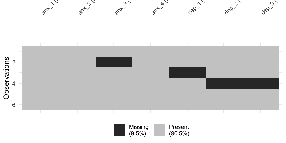
Its visualizations are often the quickest way to get an overview of the missingness in a data set. `vis_miss()` plots each cell of the data frame, with participants as rows and items as columns, showing which values are missing:
```{r}
#| fig-height: 3
#| fig-width: 6
dat_survey_na %>%
  select(starts_with("anx_"), starts_with("dep_")) %>%
  vis_miss()
```
In a real data set with hundreds of participants, this can quickly reveal patterns, e.g., if missingness is concentrated in one scale, one item, or a subset of participants who dropped out partway through the study.
#### Deciding how to handle missing data
A common rule, which should ideally be stated in your preregistration, is to calculate a participant's score only if they have *no* missing data. This is what `rowSums()` and `rowMeans()` do by default, but it can be useful to make the rule explicit in your code:
```{r}
dat_survey_missingness %>%
  mutate(anx_mean = rowMeans(pick(anx_1, anx_2_reversed, anx_3, anx_4_reversed)),
         anx_mean = if_else(anx_n_missing == 0, anx_mean, NA_real_)) %>%
  select(id, anx_n_missing, anx_mean) %>%
  kable() %>%
  kable_classic(full_width = FALSE)
```
This is simple and transparent, but it can throw away a lot of data: a participant who answered 19 of 20 items gets no score at all. There are two common alternatives.
**Mean imputation within each participant.** Calculate each participant's score from the items they *did* answer, usually only if they are missing no more than a small number of items. For mean scores, this is just `rowMeans(..., na.rm = TRUE)`. For sum scores, multiply the participant's mean by the total number of items in the scale, so that the score remains on the same scale as everyone else's (unlike `rowSums(..., na.rm = TRUE)`, which treats missing responses as 0):
```{r}
dat_survey_missingness %>%
  mutate(anx_mean_imputed = rowMeans(pick(anx_1, anx_2_reversed, anx_3, anx_4_reversed), na.rm = TRUE),
         anx_sum_imputed = anx_mean_imputed * 4, # 4 items in the scale
         # only calculate scores for participants missing no more than one item
         anx_mean_imputed = if_else(anx_n_missing <= 1, anx_mean_imputed, NA_real_),
         anx_sum_imputed = if_else(anx_n_missing <= 1, anx_sum_imputed, NA_real_)) %>%
  select(id, anx_n_missing, anx_mean_imputed, anx_sum_imputed) %>%
  kable() %>%
  kable_classic(full_width = FALSE)
```
This is often defensible: if the items of a scale measure the same thing, a participant's responses to the items they answered are a reasonable estimate of what they would have answered on the item they skipped.
What is *not* usually defensible is imputing *across* participants, e.g., replacing a participant's missing response or score with the sample mean. This makes participants with missing data look artificially average, which artificially reduces the variance in the data and biases correlations and effect sizes. If you need to deal with missing data across participants, use methods designed for it, such as multiple imputation (e.g., with the {mice} package), which are beyond the scope of this book.
**Requiring responses to every item.** Many survey platforms let you make every item mandatory, so that there is no item-level missing data to deal with in the first place. This makes processing simpler, but has downsides: participants who don't want to answer an item may give a random or false response instead, or quit the study entirely, which just moves the missing data from the item level to the participant level, where it's harder to deal with. Ethics committees may also require that participants be allowed to skip questions they don't want to answer. A common compromise is to require a response but include a "prefer not to answer" option, which of course then needs to be converted to `NA` during processing.
Whichever approach you choose, decide on it before seeing the data, state it in your preregistration, and implement it explicitly in your code.
#### Doing it all at once with a wrapper: `snuffle_sum_scores()`
Everything in this section, i.e., setting impossible values to `NA`, reverse scoring, counting missing items, and calculating (optionally imputed) sum scores, is so commonly needed that the {truffle} package provides a wrapper function that does all of it: `snuffle_sum_scores()`.
Note that it is applied to the raw 'dat_survey' data: the `-99` codes are outside the 1-5 range of the scale (`min` and `max`), so they are treated as impossible values and set to `NA`.
```{r}
# install.packages("devtools"); devtools::install_github("ianhussey/truffle")
library(truffle)

dat_survey %>%
  snuffle_sum_scores(scale_identifier = "anx_", # the prefix of the scale's item columns
                     min = 1, # lowest possible response
                     max = 5, # highest possible response
                     reverse = c("anx_2", "anx_4"), # reverse-keyed items
                     impute = TRUE, # impute sum scores from each participant's mean
                     id_col = "id") %>% # checks that there are no duplicate ids
  select(id, starts_with("anx_")) %>%
  kable() %>%
  kable_classic(full_width = FALSE)
```
The 'anx_sumscore' column matches the 'anx_sum_imputed' column calculated by hand above. It also returns columns that help you check what it did, e.g., how many items were present for each participant ('anx_nonmissing_n'), how many impossible values were found ('anx_impossible_n'), and which items were reversed ('anx_items_reversed').
Two things to note. First, `impute = TRUE` imputes sum scores for participants missing *any* number of items, so you would still need to apply your own rule about how many missing items are acceptable, e.g., using 'anx_nonmissing_n'. Second, it overwrites the reverse-keyed item columns with their reversed scores, which, as discussed above, makes it harder to check that reversing was done correctly. As with any wrapper, it's worth understanding the logic it implements, which you now do, so that you can check that it does what you need.
### Exercise
Using 'dat_survey_na' (where the `-99`s have already been converted to `NA`), write code that:
- Calculates each participant's mean depression score, using only the items they responded to.
- Counts how many depression items each participant is missing.
- Creates a final column 'dep_mean_final' that contains the mean score if the participant was missing no more than one item, and `NA` otherwise.
- Prints the id column and the new columns.
```{r}
#| include: false
```
::: {.callout-note collapse="true" title="Click to show answer"}
```{r}
dat_survey_na %>%
  mutate(dep_mean_na_rm = rowMeans(pick(dep_1, dep_2, dep_3), na.rm = TRUE),
         dep_n_missing = rowSums(is.na(pick(dep_1, dep_2, dep_3))),
         dep_mean_final = if_else(dep_n_missing <= 1, dep_mean_na_rm, NA_real_)) %>%
  select(id, dep_mean_na_rm, dep_n_missing, dep_mean_final) %>%
  kable() %>%
  kable_classic(full_width = FALSE)
```
Participant 4 is missing two of the three depression items, so their final score is `NA`, even though `rowMeans(..., na.rm = TRUE)` calculated a score from their single remaining response.
:::
## Using values from other rows: `lag()` and `lead()`
So far, every `mutate()` has calculated a value using other values in the *same row*. Sometimes we need values from *other rows*. This is common in trial-level data from experiments, where each row is a trial and the order of the trials matters.
- `lag(x)` returns the value of x in the *previous* row.
- `lead(x)` returns the value of x in the *next* row.
For example, here is one participant's data from a reaction time task, where 'correct' is 1 for correct responses and 0 for errors:
```{r}
dat_trials <- tribble(
  ~id, ~trial, ~rt, ~correct,
  1,   1,      650, 1,
  1,   2,      590, 1,
  1,   3,      720, 0,
  1,   4,      810, 1,
  1,   5,      600, 1,
  1,   6,      580, 0,
  1,   7,      760, 1,
  1,   8,      640, 1
)

dat_trials %>%
  mutate(rt_previous = lag(rt),
         rt_next = lead(rt),
         correct_previous = lag(correct)) %>%
  kable() %>%
  kable_classic(full_width = FALSE)
```
The first row has no previous row, so `lag()` returns `NA` there. Likewise, the last row has no next row, so `lead()` returns `NA`.
A well-known phenomenon in reaction time tasks is "post-error slowing": people tend to respond more slowly on the trial immediately after making an error. To study this, we need to know whether each trial came after an error, which requires `lag()`:
```{r}
dat_trials %>%
  mutate(after_error = if_else(lag(correct) == 0, "post-error", "post-correct")) %>%
  kable() %>%
  kable_classic(full_width = FALSE)
```
Trials 4 and 7 came after an error, and indeed have longer RTs. Trial 1 is `NA` as it has no previous trial.
### Row order matters
`lag()` and `lead()` use the order of the rows in the data frame, not the trial number. If the data are not in the correct order, the results will be silently wrong. It's therefore good practice to `arrange()` the data before using them:
```{r}
dat_trials %>%
  # put the rows in the wrong order, as an example
  arrange(desc(rt)) %>%
  # arrange by trial before using lag()
  arrange(trial) %>%
  mutate(correct_previous = lag(correct)) %>%
  kable() %>%
  kable_classic(full_width = FALSE)
```
### Watch out when there are multiple participants
`lag()` and `lead()` don't know anything about participants. If a data frame contains several participants' data, the first trial of participant 2 will be given the last trial of participant 1 as its "previous" trial:
```{r}
dat_trials_two_participants <- tribble(
  ~id, ~trial, ~rt, ~correct,
  1,   1,      650, 1,
  1,   2,      590, 1,
  1,   3,      720, 0,
  2,   1,      880, 1,
  2,   2,      910, 0,
  2,   3,      1020, 1
)

dat_trials_two_participants %>%
  arrange(id, trial) %>%
  mutate(correct_previous = lag(correct)) %>%
  kable() %>%
  kable_classic(full_width = FALSE)
```
Participant 2's first trial should be `NA`, but it has been given the value of participant 1's last trial. In the next chapter, you'll learn about `group_by()`, which solves this problem by making functions like `lag()` operate separately within each participant.
### Running counts: `row_number()` and `cumsum()`
Two other functions that depend on row order are also useful here:
- `row_number()` returns the row number, 1, 2, 3, etc. This is useful when a data set doesn't contain a trial number column.
- `cumsum()` returns the cumulative (running) sum. When used with a logical test, it counts how many times the test has been TRUE so far.
```{r}
dat_trials %>%
  mutate(row = row_number(),
         n_errors_so_far = cumsum(correct == 0)) %>%
  kable() %>%
  kable_classic(full_width = FALSE)
```
### Exercise
Using 'dat_trials', write code that creates:
- 'rt_change' : the difference between the RT on each trial and the RT on the previous trial.
- 'next_trial_error' : TRUE if the *next* trial was an error, and FALSE otherwise.
```{r}
#| include: false
```
::: {.callout-note collapse="true" title="Click to show answer"}
```{r}
dat_trials %>%
  arrange(trial) %>%
  mutate(rt_change = rt - lag(rt),
         next_trial_error = lead(correct) == 0) %>%
  kable() %>%
  kable_classic(full_width = FALSE)
```
:::
## Filling in empty cells with `fill()`
Data that has been entered or edited by hand, e.g., in Excel, often only writes a value the first time it appears, leaving the cells below it empty to make it easier to read. For example, the participant id and block are only written on the first row they apply to:
```{r}
dat_excel <- tribble(
  ~id, ~block,     ~trial, ~rt,
  1,   "practice", 1,      812,
  NA,  NA,         2,      1043,
  NA,  "test",     1,      612,
  NA,  NA,         2,      788,
  2,   "practice", 1,      1150,
  NA,  NA,         2,      1320,
  NA,  "test",     1,      760,
  NA,  NA,         2,      655
)

dat_excel %>%
  kable() %>%
  kable_classic(full_width = FALSE)
```
This is easy for a human to read but makes the data much harder to work with in R. For example, `filter(id == 2)` would return only one row.
{tidyr}'s `fill()` fills in missing values with the last non-missing value above them:
```{r}
dat_excel %>%
  fill(id, block) %>%
  kable() %>%
  kable_classic(full_width = FALSE)
```
By default `fill()` fills downwards. You can change this with the `.direction` argument, e.g., `.direction = "up"` if the value is written on the last row of each set rather than the first.
`fill()` should only be used when you know that `NA` means "same as the row above". If a value is genuinely missing, e.g., participant 2's first block label was never recorded, `fill()` would silently give it participant 1's block label. As with `lag()`, `fill()` doesn't know about participants on its own; `group_by()`, covered in the next chapter, can be used to make it fill within each participant only.
### Exercise
The following data has one row per item of a questionnaire, but the 'scale' column is only filled in on the last row of each scale. Use `fill()` to fill in the 'scale' column correctly.
```{r}
dat_items <- tribble(
  ~item, ~scale,       ~response,
  1,     NA,           3,
  2,     NA,           4,
  3,     "anxiety",    2,
  1,     NA,           5,
  2,     NA,           4,
  3,     "depression", 4
)
```
```{r}
#| include: false
```
::: {.callout-note collapse="true" title="Click to show answer"}
```{r}
dat_items %>%
  fill(scale, .direction = "up") %>%
  kable() %>%
  kable_classic(full_width = FALSE)
```
:::
## Separating one column into several or coalescing several columns into one
Another common task is splitting one column into several, e.g., a column containing "anx_1" into a column for the scale ("anx") and one for the item number ("1"). This is done with `separate()`.
The opposite task is combining several columns into one, e.g., when age was saved in a different column in each version of a survey, and you want a single 'age' column containing whichever value is not missing. This is done with `coalesce()`.
Both are covered in the [Reshaping and pivots](12_reshaping_and_pivots.qmd) chapter, as they are about changing the structure of the data rather than just its contents.
## Exercises
### `arrange()` and missing values
When you use `arrange(desc(x))` on a column containing `NA`s, where do the `NA`s go?
::: {.callout-note collapse="true" title="Click to show answer"}
At the end. `arrange()` always puts `NA`s last, whether the order is ascending or descending.
:::
### `slice_max()` and ties
You run `slice_max(score, n = 3)` and get four rows back. Why?
::: {.callout-note collapse="true" title="Click to show answer"}
Two or more rows are tied for third place. By default, `slice_min()` and `slice_max()` keep ties (`with_ties = TRUE`).
:::
### `drop_na()`
What is the difference between `drop_na()` and `drop_na(age)`? Which should you usually use and why?
::: {.callout-note collapse="true" title="Click to show answer"}
`drop_na()` drops every row with an `NA` in *any* column. `drop_na(age)` drops only rows where 'age' is `NA`. It's usually better to be explicit and name the column(s), so that rows aren't dropped because of missing values in columns that aren't relevant to your analysis.
:::
### Missing data codes
What functions could you use to convert a missing data code like `-99` into `NA`? Why must this be done before any calculations?
::: {.callout-note collapse="true" title="Click to show answer"}
`if_else(x == -99, NA_real_, x)` or the shortcut `na_if(x, -99)`. If it isn't done, R treats `-99` as a real number, and calculations like means will be wrong without any error or warning.
:::
### `across()`
What are the two main arguments of `across()`, and what does each one do? What do `~` and `.x` mean?
::: {.callout-note collapse="true" title="Click to show answer"}
- `.cols` : which columns to apply the function to. This uses the same syntax as `select()`, including the {tidyselect} helper functions.
- `.fns` : the function to apply to each of those columns.
`~` indicates that you are writing a function on the fly, and `.x` is a placeholder for "the current column".
:::
How would you use `across()` to create new columns rather than overwriting the existing ones?
::: {.callout-note collapse="true" title="Click to show answer"}
With the `.names` argument, e.g., `.names = "{.col}_reversed"`, where `{.col}` is replaced with the name of the original column.
:::
### Scores across columns
Why does `mutate(total = sum(item_1, item_2, item_3))` not calculate each participant's total score? What could you use instead?
::: {.callout-note collapse="true" title="Click to show answer"}
`sum()` is an aggregating function. It adds up all the values in all three columns across all rows into one number, which is then repeated in every row. Instead, use `item_1 + item_2 + item_3`, or `rowSums(pick(item_1, item_2, item_3))`, which calculate within each row.
:::
Why can using `rowSums(..., na.rm = TRUE)` be problematic for calculating sum scores?
::: {.callout-note collapse="true" title="Click to show answer"}
It sums only the items that are present, which effectively treats missing responses as 0. Participants with missing responses will have artificially low scores that are not comparable with participants with complete data.
:::
### `lag()` and `lead()`
What do `lag()` and `lead()` do? Name two things that can make their results silently wrong.
::: {.callout-note collapse="true" title="Click to show answer"}
`lag()` returns the value from the previous row and `lead()` returns the value from the next row.
- The rows are not in the right order, e.g., not arranged by trial number. Use `arrange()` first.
- The data frame contains multiple participants, so the first row of one participant is given values from the last row of the previous participant. This can be solved with `group_by()`, covered in the next chapter.
:::
### `fill()`
When is it appropriate to use `fill()`, and when is it not?
::: {.callout-note collapse="true" title="Click to show answer"}
It's appropriate when an `NA` means "the same value as the row above (or below)", e.g., in hand-entered data where an ID is only written on the first row of each participant. It's not appropriate when values are genuinely missing, as `fill()` would replace them with another row's value.
:::
### Interactive exercises
Complete the interactive exercises for:
- [`across()`](https://errors.shinyapps.io/dplyr-learnr/#section-dplyracross)
### Practice data transformation using multiple functions
In your local version of this .qmd file:
- Use 'dat_survey' to create a new data frame called 'dat_survey_processed'.
- Convert all `-99`s to `NA`, without modifying the 'id' column.
- Reverse score anxiety items 2 and 4 into new columns.
- Calculate each participant's mean anxiety score and mean depression score, and the number of missing items for each scale.
- Set each mean score to `NA` if the participant was missing more than one item on that scale.
- Keep only the 'id', 'age', 'condition' columns and the final score columns.
- Arrange the data frame from the highest to the lowest anxiety score.
- Print the data frame as a table.
```{r}
#| include: false
```