add content on in-text results reporting and using LLMs to aid writing them.
16.2 Dependencies
library(dplyr)library(readr)library(report) # part of {easystats}library(see) # part of {easystats}library(parameters) # part of {easystats}library(correlation) # part of {easystats}library(effectsize) # part of {easystats}library(performance) # part of {easystats}library(janitor)library(lme4)library(knitr)library(kableExtra)
16.3 Inference tests
16.3.1 Regressions
# fit modelmodel <-lm(wt ~1+ am + mpg, data = mtcars)# report - text output (nb omits intercept!)report(model)
We fitted a linear model (estimated using OLS) to predict wt with am and mpg
(formula: wt ~ 1 + am + mpg). The model explains a statistically significant
and substantial proportion of variance (R2 = 0.80, F(2, 29) = 57.66, p < .001,
adj. R2 = 0.79). The model's intercept, corresponding to am = 0 and mpg = 0, is
at 5.74 (95% CI [5.11, 6.36], t(29) = 18.64, p < .001). Within this model:

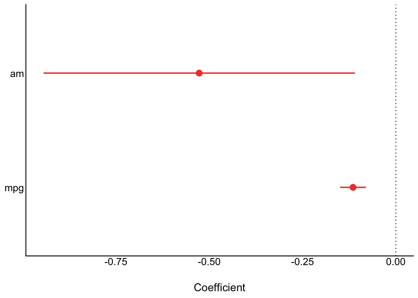
  - The effect of am is statistically significant and negative (beta = -0.53, 95%
CI [-0.94, -0.11], t(29) = -2.58, p = 0.015; Std. beta = -0.27, 95% CI [-0.48,
-0.06])
  - The effect of mpg is statistically significant and negative (beta = -0.11,
95% CI [-0.15, -0.08], t(29) = -6.79, p < .001; Std. beta = -0.71, 95% CI
[-0.92, -0.49])

Standardized parameters were obtained by fitting the model on a standardized
version of the dataset. 95% Confidence Intervals (CIs) and p-values were
computed using a Wald t-distribution approximation.
# each parameter (including intercept)report_parameters(model)
  - The intercept is statistically significant and positive (beta = 5.74, 95% CI [5.11, 6.36], t(29) = 18.64, p < .001; Std. beta = 7.12e-17, 95% CI [-0.17, 0.17])
  - The effect of am is statistically significant and negative (beta = -0.53, 95% CI [-0.94, -0.11], t(29) = -2.58, p = 0.015; Std. beta = -0.27, 95% CI [-0.48, -0.06])
  - The effect of mpg is statistically significant and negative (beta = -0.11, 95% CI [-0.15, -0.08], t(29) = -6.79, p < .001; Std. beta = -0.71, 95% CI [-0.92, -0.49])
# just parameters in text formatreport_statistics(model)
beta = 5.74, 95% CI [5.11, 6.36], t(29) = 18.64, p < .001; Std. beta = 7.12e-17, 95% CI [-0.17, 0.17]
beta = -0.53, 95% CI [-0.94, -0.11], t(29) = -2.58, p = 0.015; Std. beta = -0.27, 95% CI [-0.48, -0.06]
beta = -0.11, 95% CI [-0.15, -0.08], t(29) = -6.79, p < .001; Std. beta = -0.71, 95% CI [-0.92, -0.49]
# just parameters in table formatparameters(model)
Parameter
Coefficient
SE
CI
CI_low
CI_high
t
df_error
p
(Intercept)
5.7355639
0.3077263
0.95
5.1061930
6.3649348
18.638525
29
0.0000000
am
-0.5269568
0.2039939
0.95
-0.9441712
-0.1097424
-2.583199
29
0.0150986
mpg
-0.1146922
0.0168893
0.95
-0.1492347
-0.0801496
-6.790807
29
0.0000002
# just parameters in table html format parameters(model) |>mutate(p = insight::format_p(p)) |>mutate_if(is.numeric, round_half_up, digits =2) |>kable() |>kable_classic(full_width =FALSE)
Parameter
Coefficient
SE
CI
CI_low
CI_high
t
df_error
p
(Intercept)
5.74
0.31
0.95
5.11
6.36
18.64
29
p < .001
am
-0.53
0.20
0.95
-0.94
-0.11
-2.58
29
p = 0.015
mpg
-0.11
0.02
0.95
-0.15
-0.08
-6.79
29
p < .001
# what if i just want some of these cols?parameters(model) |>as.data.frame() |>mutate(p = insight::format_p(p)) |>select(r = Coefficient, ci_lower = CI_low, ci_upper = CI_high, p) |>mutate_if(is.numeric, round_half_up, digits =2)
r
ci_lower
ci_upper
p
5.74
5.11
6.36
p < .001
-0.53
-0.94
-0.11
p = 0.015
-0.11
-0.15
-0.08
p < .001
# table in markdown formatreport_table(model)
Parameter
Coefficient
CI
CI_low
CI_high
t
df_error
p
Std_Coefficient
Std_Coefficient_CI_low
Std_Coefficient_CI_high
Fit
1
(Intercept)
5.7355639
0.95
5.1061930
6.3649348
18.638525
29
0.0000000
0.0000000
-0.1675614
0.1675614
NA
2
am
-0.5269568
0.95
-0.9441712
-0.1097424
-2.583199
29
0.0150986
-0.2687359
-0.4815057
-0.0559661
NA
3
mpg
-0.1146922
0.95
-0.1492347
-0.0801496
-6.790807
29
0.0000002
-0.7064629
-0.9192327
-0.4936930
NA
4
NA
NA
NA
NA
NA
NA
NA
NA
NA
NA
NA
NA
5
AIC
NA
NA
NA
NA
NA
NA
NA
NA
NA
NA
45.0491609
6
AICc
NA
NA
NA
NA
NA
NA
NA
NA
NA
NA
46.5306424
7
BIC
NA
NA
NA
NA
NA
NA
NA
NA
NA
NA
50.9121045
8
R2
NA
NA
NA
NA
NA
NA
NA
NA
NA
NA
0.7990675
9
R2 (adj.)
NA
NA
NA
NA
NA
NA
NA
NA
NA
NA
0.7852101
11
Sigma
NA
NA
NA
NA
NA
NA
NA
NA
NA
NA
0.4534704
# table in html format - needs to be rounded manuallyreport_table(model) |>mutate(p = insight::format_p(p)) |>mutate_if(is.numeric, round_half_up, digits =2) |>kable() |>kable_classic(full_width =FALSE)
Parameter
Coefficient
CI
CI_low
CI_high
t
df_error
p
Std_Coefficient
Std_Coefficient_CI_low
Std_Coefficient_CI_high
Fit
1
(Intercept)
5.74
0.95
5.11
6.36
18.64
29
p < .001
0.00
-0.17
0.17
NA
2
am
-0.53
0.95
-0.94
-0.11
-2.58
29
p = 0.015
-0.27
-0.48
-0.06
NA
3
mpg
-0.11
0.95
-0.15
-0.08
-6.79
29
p < .001
-0.71
-0.92
-0.49
NA
4
NA
NA
NA
NA
NA
NA
NA
NA
NA
NA
NA
5
AIC
NA
NA
NA
NA
NA
NA
NA
NA
NA
45.05
6
AICc
NA
NA
NA
NA
NA
NA
NA
NA
NA
46.53
7
BIC
NA
NA
NA
NA
NA
NA
NA
NA
NA
50.91
8
R2
NA
NA
NA
NA
NA
NA
NA
NA
NA
0.80
9
R2 (adj.)
NA
NA
NA
NA
NA
NA
NA
NA
NA
0.79
11
Sigma
NA
NA
NA
NA
NA
NA
NA
NA
NA
0.45
# plotparameters(model) |>plot()
16.3.2 Correlations
16.3.2.1 Single correlation tests
# fit modelmodel <-cor.test(mtcars$mpg, mtcars$wt)# report - text output report(model)
Effect sizes were labelled following Funder's (2019) recommendations.

The Pearson's product-moment correlation between mtcars$mpg and mtcars$wt is
negative, statistically significant, and very large (r = -0.87, 95% CI [-0.93,
-0.74], t(30) = -9.56, p < .001)
# table in html format - needs to be rounded manuallyreport_table(model) |>mutate(p = insight::format_p(p)) |>mutate_if(is.numeric, round_half_up, digits =2) |>kable() |>kable_classic(full_width =FALSE)
NB Cohen’s d is approximated - better to calculate it separately and accurately.
# fit modelmodel <-t.test(mpg ~ am, data = mtcars)# report - text output report(model)
Effect sizes were labelled following Cohen's (1988) recommendations.

The Welch Two Sample t-test testing the difference of mpg by am (mean in group
0 = 17.15, mean in group 1 = 24.39) suggests that the effect is negative,
statistically significant, and large (difference = -7.24, 95% CI [-11.28,
-3.21], t(18.33) = -3.77, p = 0.001; Cohen's d = -1.76, 95% CI [-2.82, -0.67])
# table in html format - needs to be rounded manuallyreport_table(model) |>mutate(p = insight::format_p(p)) |>mutate_if(is.numeric, round_half_up, digits =2) |>kable() |>kable_classic(full_width =FALSE)
Parameter
Group
Mean_Group1
Mean_Group2
Difference
CI
CI_low
CI_high
t
df_error
p
Method
Alternative
d
d_CI_low
d_CI_high
mpg
am
17.15
24.39
-7.24
0.95
-11.28
-3.21
-3.77
18.33
p = 0.001
Welch Two Sample t-test
two.sided
-1.76
-2.82
-0.67
# estimate Cohen's d directly from datacohens_d(mpg ~ am, data = mtcars)
Cohens_d
CI
CI_low
CI_high
-1.477947
0.95
-2.265973
-0.6705684
16.3.4 Multilevel/hierarchical/mixed models
# fit modelmodel <-lmer(Reaction ~ Days + (Days | Subject), sleepstudy)# parameters in text format report(model)
We fitted a linear mixed model (estimated using REML and nloptwrap optimizer)
to predict Reaction with Days (formula: Reaction ~ Days). The model included
Days as random effects (formula: ~Days | Subject). The model's total
explanatory power is substantial (conditional R2 = 0.80) and the part related
to the fixed effects alone (marginal R2) is of 0.28. The model's intercept,
corresponding to Days = 0, is at 251.41 (95% CI [237.94, 264.87], t(174) =
36.84, p < .001). Within this model:

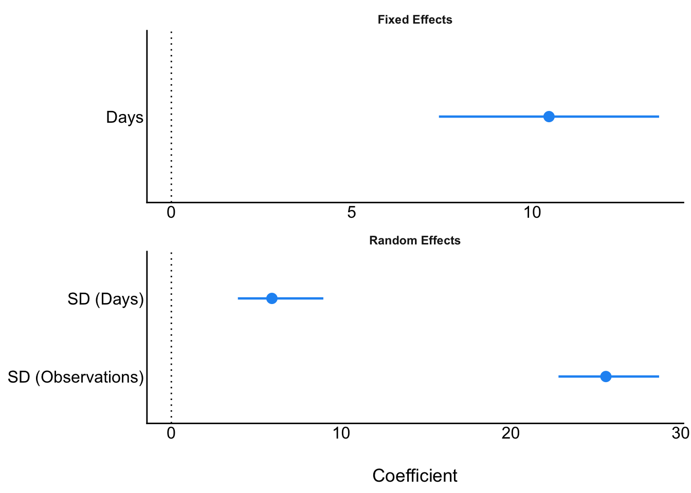
  - The effect of Days is statistically significant and positive (beta = 10.47,
95% CI [7.42, 13.52], t(174) = 6.77, p < .001; Std. beta = 0.54, 95% CI [0.38,
0.69])

Standardized parameters were obtained by fitting the model on a standardized
version of the dataset. 95% Confidence Intervals (CIs) and p-values were
computed using a Wald t-distribution approximation.
# table in html format - needs to be rounded manuallyreport_table(model) |>mutate(p = insight::format_p(p)) |>mutate_if(is.numeric, round_half_up, digits =2) |>kable() |>kable_classic(full_width =FALSE)
Parameter
Coefficient
CI
CI_low
CI_high
t
df_error
p
Effects
Group
Std_Coefficient
Std_Coefficient_CI_low
Std_Coefficient_CI_high
Fit
1
(Intercept)
251.41
0.95
237.94
264.87
36.84
174
p < .001
fixed
0.00
-0.32
0.32
NA
2
Days
10.47
0.95
7.42
13.52
6.77
174
p < .001
fixed
0.54
0.38
0.69
NA
3
NA
24.74
0.95
NA
NA
NA
NA
random
Subject
NA
NA
NA
NA
4
NA
5.92
0.95
NA
NA
NA
NA
random
Subject
NA
NA
NA
NA
5
NA
0.07
0.95
NA
NA
NA
NA
random
Subject
NA
NA
NA
NA
6
NA
25.59
0.95
NA
NA
NA
NA
random
Residual
NA
NA
NA
NA
7
NA
NA
NA
NA
NA
NA
NA
NA
NA
NA
NA
NA
NA
8
AIC
NA
NA
NA
NA
NA
NA
NA
NA
NA
NA
NA
1755.63
9
AICc
NA
NA
NA
NA
NA
NA
NA
NA
NA
NA
NA
1756.11
10
BIC
NA
NA
NA
NA
NA
NA
NA
NA
NA
NA
NA
1774.79
11
R2 (conditional)
NA
NA
NA
NA
NA
NA
NA
NA
NA
NA
NA
0.80
12
R2 (marginal)
NA
NA
NA
NA
NA
NA
NA
NA
NA
NA
NA
0.28
15
Sigma
NA
NA
NA
NA
NA
NA
NA
NA
NA
NA
NA
25.59
# plotparameters(model) |>plot()
# check assumptions of random effectsresult <-check_normality(model, effects ="random")plot(result)
[[1]]
16.3.5 ANOVAs
# fit modelmodel <-aov(mpg ~factor(gear) +factor(carb), data = mtcars)# commonly used effect size: partial eta squaredeta_squared(model)
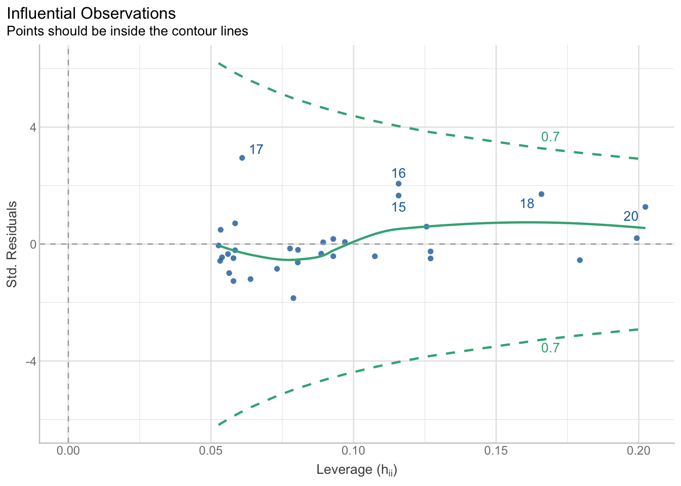
res_outliers <-check_outliers(model, method ="cook") # "all" requires other dependencies and can take some time to run #res_outliers <- check_outliers(model, method = "all") # "all" requires other dependencies and can take some time to run res_outliers
OK: No outliers detected.
- Based on the following method and threshold: cook (0.808).
- For variable: (Whole model)
plot(res_outliers)
16.5.5 Heteroscedasticity
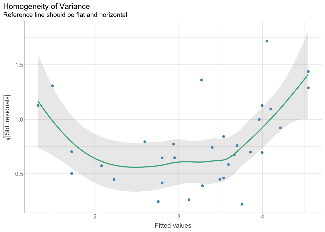
res_het <-check_heteroscedasticity(model)res_het
OK: Error variance appears to be homoscedastic (p = 0.053).
plot(res_het)
Source Code
# Reporting <span class="badge badge-draft3">✎ Small TODOs</span>## TODOadd content on in-text results reporting and using LLMs to aid writing them. ```{r}#| include: false# settings, placed in a chunk that will not show in the .html file (because include=FALSE) # disables scientific notation so that small numbers appear as eg "0.00001" rather than "1e-05"options(scipen =999) ```## Dependencies```{r}library(dplyr)library(readr)library(report) # part of {easystats}library(see) # part of {easystats}library(parameters) # part of {easystats}library(correlation) # part of {easystats}library(effectsize) # part of {easystats}library(performance) # part of {easystats}library(janitor)library(lme4)library(knitr)library(kableExtra)```## Inference tests### Regressions```{r}# fit modelmodel <-lm(wt ~1+ am + mpg, data = mtcars)# report - text output (nb omits intercept!)report(model)# each parameter (including intercept)report_parameters(model)# just parameters in text formatreport_statistics(model)# just parameters in table formatparameters(model)# just parameters in table html format parameters(model) |>mutate(p = insight::format_p(p)) |>mutate_if(is.numeric, round_half_up, digits =2) |>kable() |>kable_classic(full_width =FALSE)# what if i just want some of these cols?parameters(model) |>as.data.frame() |>mutate(p = insight::format_p(p)) |>select(r = Coefficient, ci_lower = CI_low, ci_upper = CI_high, p) |>mutate_if(is.numeric, round_half_up, digits =2)# table in markdown formatreport_table(model)# table in html format - needs to be rounded manuallyreport_table(model) |>mutate(p = insight::format_p(p)) |>mutate_if(is.numeric, round_half_up, digits =2) |>kable() |>kable_classic(full_width =FALSE)# plotparameters(model) |>plot() ```### Correlations#### Single correlation tests```{r}# fit modelmodel <-cor.test(mtcars$mpg, mtcars$wt)# report - text output report(model)# table in html format - needs to be rounded manuallyreport_table(model) |>mutate(p = insight::format_p(p)) |>mutate_if(is.numeric, round_half_up, digits =2) |>kable() |>kable_classic(full_width =FALSE)```#### Many```{r}results <-correlation(iris)resultsresults %>%summary(redundant =TRUE) %>%plot()```#### By group```{r}iris %>%select(Species, Sepal.Length, Sepal.Width, Petal.Width) %>%group_by(Species) %>%correlation()```### t-testsNB Cohen's d is approximated - better to calculate it separately and accurately.```{r}# fit modelmodel <-t.test(mpg ~ am, data = mtcars)# report - text output report(model)# table in html format - needs to be rounded manuallyreport_table(model) |>mutate(p = insight::format_p(p)) |>mutate_if(is.numeric, round_half_up, digits =2) |>kable() |>kable_classic(full_width =FALSE)# estimate Cohen's d directly from datacohens_d(mpg ~ am, data = mtcars)```### Multilevel/hierarchical/mixed models```{r}# fit modelmodel <-lmer(Reaction ~ Days + (Days | Subject), sleepstudy)# parameters in text format report(model)# parameters in table formatparameters(model) |>mutate(p = insight::format_p(p)) |>mutate_if(is.numeric, round_half_up, digits =2) |>kable() |>kable_classic(full_width =FALSE)# table in html format - needs to be rounded manuallyreport_table(model) |>mutate(p = insight::format_p(p)) |>mutate_if(is.numeric, round_half_up, digits =2) |>kable() |>kable_classic(full_width =FALSE)# plotparameters(model) |>plot() # check assumptions of random effectsresult <-check_normality(model, effects ="random")plot(result)```### ANOVAs```{r}# fit modelmodel <-aov(mpg ~factor(gear) +factor(carb), data = mtcars)# commonly used effect size: partial eta squaredeta_squared(model)# better effect size: partialomega squaredomega_squared(model)```## Summary statistics```{r}# all columnsiris |>group_by(Species) |>report_table() # all columns - html output with roundingiris |>group_by(Species) |>report_table() |>mutate_if(is.numeric, round_half_up, digits =2) |>kable() |>kable_classic(full_width =FALSE)# subset of columnsiris |>group_by(Species) |>report_table() |>select(Group, Variable, n_Obs, Mean, SD) |>mutate_if(is.numeric, round_half_up, digits =2) |>kable() |>kable_classic(full_width =FALSE)```## Assumption checksBeware that checking assumptions can lead to as many bad practices as it does good ones! (e.g., poorly justified post hoc outlier exclusion)### Multiple checks at once```{r fig.height=8, fig.width=8}# fit modelmodel <-lm(wt ~1+ am + mpg, data = mtcars)# check multiple model assumptionscheck_model(model)```### Normality of distribution of residuals```{r}res_normality <-check_normality(model)res_normalityplot(res_normality, type ="qq")plot(res_normality, type ="density")```### Multicolinearity```{r}res_collinearity <-check_collinearity(model)res_collinearityplot(res_collinearity)```### Outliers```{r}res_outliers <-check_outliers(model, method ="cook") # "all" requires other dependencies and can take some time to run #res_outliers <- check_outliers(model, method = "all") # "all" requires other dependencies and can take some time to run res_outliersplot(res_outliers)```### Heteroscedasticity```{r}res_het <-check_heteroscedasticity(model)res_hetplot(res_het)```