2  Fundamentals

2.1 What’s the difference between Base R, RStudio IDE, and tidyverse?

This is an understandable point of confusion, so let’s clarify:

• Base R is the coding language that we learn in this course.
• RStudio IDE (Integrated Development Environment) is the application we use to write R code in. There are others but RStudio is the best option, although this could change in future.
• {tidyverse} is a set of R packages that enhance base R’s utility and usability, built around the concept of Tidy Data. We’ll learn about Tidy Data in another chapter. {tidyverse} arguably changes how we write R code so fundamentally that some people argue that R+{tidyverse} should be conceptualized as a meaningfully different language with different conventions and workflows.

There is a long-standing debate about whether base R (alone) or R+{tidyverse} is better. Thankfully, I can resolve this question for you immediately: R+{tidyverse} is better. All hail the One True Language, {tidyverse}.

2.2 Scripts vs. data, console vs. source

A script is a text file that contains R code that can be re-run. Technically, you can type R code directly into the RStudio ‘Console’ and run it from there. But that would be incredibly difficult, and we want reproducible code that can be rerun, modified, and shared, so we save them in scripts. There are multiple types of scripts, including .R files (R code and comments only) as well as RMarkdown (.Rmd) and Quarto files (.qmd), which can contain code, text, plots, tables, and data. We cover these more in a later chapter on Reproducible Reports.

The RStudio interface allows you to view and write code, as well as objects that are loaded and modified by your code such as datasets. Like code scripts, datasets are also stored locally on your machine, such as in .csv and .xlsx files.

Note that you can also have text-only markdown files (.md). These can contain text and markdown formatting (e.g., bold, italics, levels of heading, etc) but not executable code. ‘Readme’ files for projects are often saved as “README.md”. .md files can be opened and edited in RStudio and also other markdown editors such as typora.io. You may need to tell your computer how to open .md file (e.g., right click>‘open with’>RStudio).

2.3 RStudio IDE basics

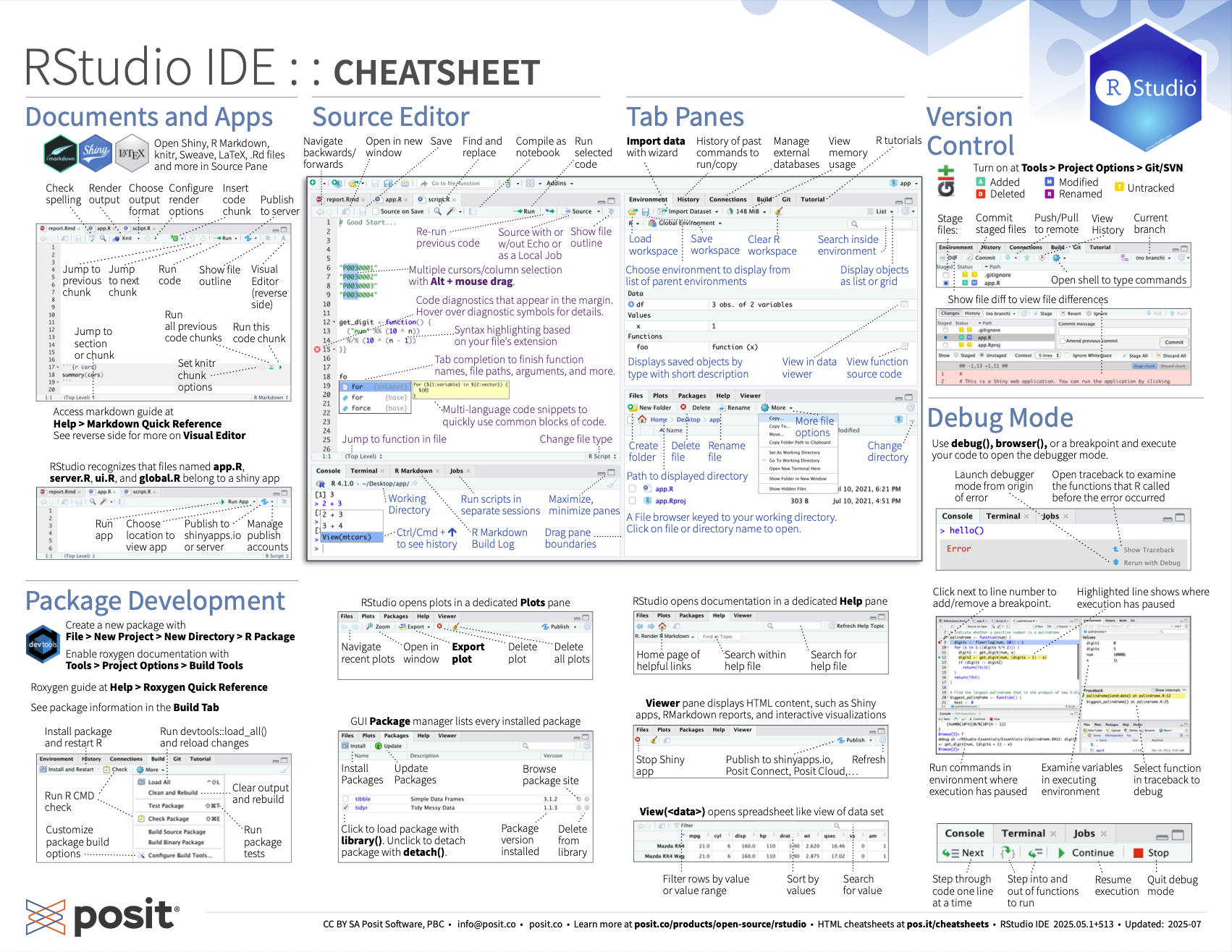
Get familiar with the different parts of the RStudio IDE user interface with this cheat-sheet, which you can also download as a pdf here.

2.3.1 Source versus Visual editor

You can view a .qmd file’s raw code in the ‘Source’ viewer. The button for this appears on the top left above the code in RStudio.

Screenshot of Source editor mode:

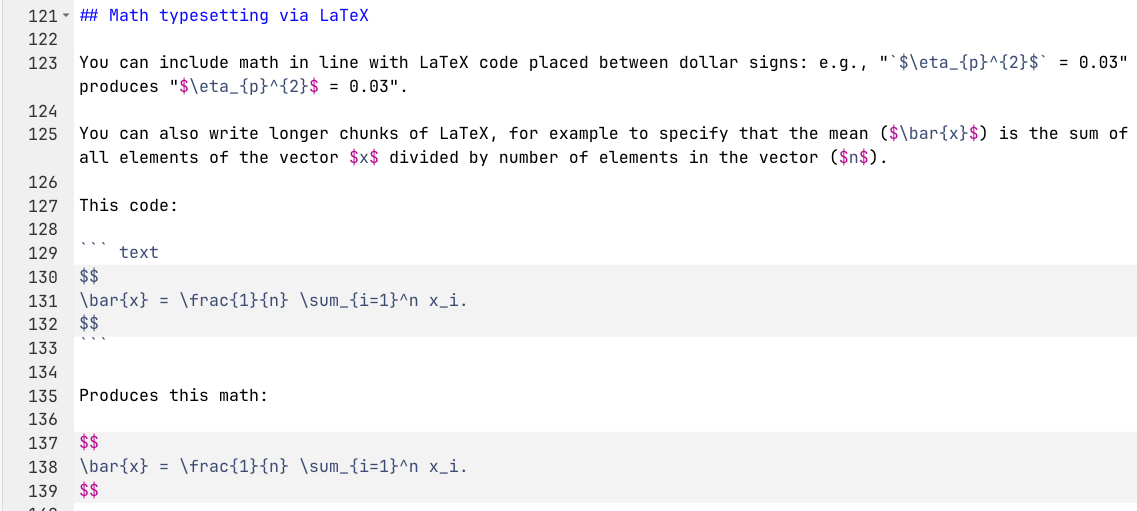
You can also view the a live preview of the rendered file, including tables, plots, math, etc., using ‘Visual’ editor mode, although there will some simplifications compared to when you render a .html file. We’ll cover rendering in a later chapter.

Screenshot of Visual editor mode:

2.3.2 Keyboard shortcuts

Once you have learned about some of the concepts mentioned below in later chapters, it can be useful to come back to these cheat-sheets to learn the keyboard shortcuts for them.

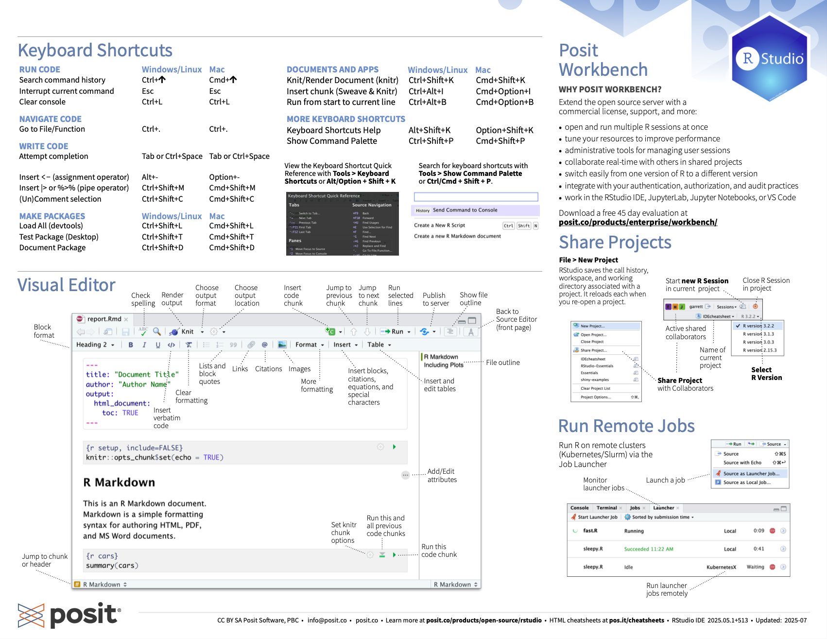
2.3.3 Particularly useful shortcuts

Windows

• Insert Chunk: Ctrl + Alt + I
• Insert Pipe (%>%): shift + Ctrl + M
• Multi-line typing: Alt + Mouse click-and-highlight multiple lines, then type
• Move cursor by word instead of by character: Alt + arrows
• Highlight words: Shift + alt + arrows
• Fix Indentation: Mouse click-and-highlight multiple lines + Ctrl + I
• Comment out (#) multiple Lines: Mouse click-and-highlight multiple lines, then Shift + Ctrl + C

Mac

• Insert Chunk: Cmd + Alt + I
• Insert Pipe (%>%): shift + Cmd + M
• Multi-line typing: Alt + Mouse click-and-highlight multiple lines, then type
• Move cursor by word instead of by character: Option + arrows
• Highlight words: Shift + option + arrows
• Fix Indentation: Mouse click-and-highlight multiple lines + Cmd + I
• Comment out (#) multiple Lines: Mouse click-and-highlight multiple lines, then Shift + Cmd + C

You can also change or set up additional keyboard shortcuts in the “Tools>Modify keyboard shortcuts” drop down menu. For example, I have modified the shortcut to switch between Source viewer vs. Visual viewer to be “Cmd + `”.

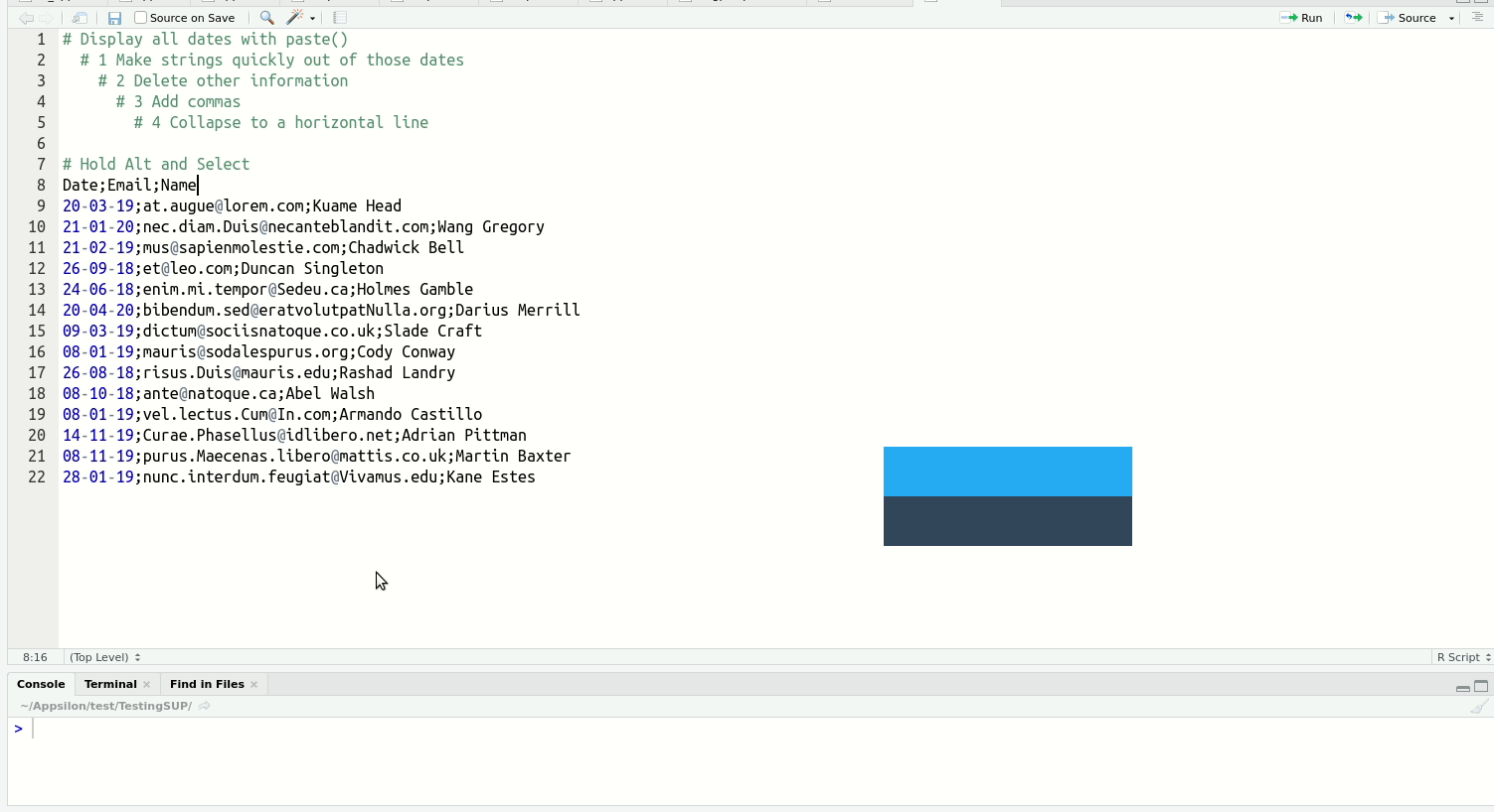
Of the above, multi-line typing is the one that reliably gets an audible ‘whoa’ from audiences. It’s easier to see than explain:

When you get a bit more experienced with RStudio, I highly recommend you check out this blog post on shortcuts to know about more advanced features such as Function/Variable Extraction, Renaming in Scope, Code Snippets, and advanced search and find-and-replace.

2.4 Dependencies

Base R includes a powerful core of many useful functions, but it doesn’t include every tool you might need. To do specialized tasks you can install ‘packages’ that contain other functions and documentation to help you understand them. Once your code makes use of another package, it ‘depends’ on that that package for the code to run, so we say that the package is a ‘dependency’ for that script. Packages that can

Install packages from the most common database of R packages, CRAN, with install.packages(). Each package only needs to be installed once for it to be present on your computer, not every time the script runs.

In your local version of this .qmd script, highlight and run the code below to install these packages.

install.packages("tidyverse") # umbrella package that installs dplyr/tidyr/ggplot2 and others
install.packages("janitor")
install.packages("report")
install.packages("parameters")
install.packages("knitr")
install.packages("kableExtra")

Some packages are instead on GitHub, and can be installed with devtools::install_github(). You’ll need to install the {devtools} package first to be able to use the install_github() function.

In your local version of this .qmd script, highlight and run the code below to install these packages.

install.packages("devtools")
devtools::install_github("ianhussey/psychdsish") # username/repository
devtools::install_github("ianhussey/truffle") # username/repository

Dependencies, i.e., packages that your code requires to run, can be loaded with library(). For tidiness, these should usually all be loaded at the start of your script. Some chapters in this book load libraries only when they’re used in order to make it clear which functions come from which libraries. Equally, unused libraries should not be loaded.

library(tidyverse) # umbrella package that loads dplyr/tidyr/ggplot2 and others

2.5 Accessing the help menu

For any function in a loaded package, simply type ? before the function’s name to bring up the help menu. This helps you understand the function’s purpose, its arguments, and outputs.

?select

If you scroll to the bottom of a function’s help page, you’ll find an ‘Index’ hyperlink. Clicking this brings you to a list of all the package’s functions. Once you get nerdy, this can be a very useful way to discover and learn all a package’s functions.

2.6 Namespace collisions: a common source of errors

Some common packages have identically named functions with different syntax. For example, if you load both {dplyr} and {MASS}, use of the function select() can refer to either dplyr::select() or MASS::select(), and your code might not run if the other package is loaded.

You can see if you have two identically named functions loaded by opening the help menu and seeing if more than one entry appears (e.g. with ?select()).

Avoid this by loading only the packages you need. Debug errors by thinking about these common namespace collisions:

Function	tidyverse Source	Conflicting Package(s)	Notes
filter	dplyr	stats	stats::filter() is for signal processing (time series)
lag	dplyr	stats	Different semantics: dplyr::lag() is simpler
select	dplyr	MASS	MASS::select() is for step-wise regression
slice	dplyr	IRanges / S4Vectors	Common in Bioconductor workflows
rename	dplyr	MASS	MASS::rename() is deprecated, but may still load
summarise	dplyr	Hmisc	Hmisc::summarize() differs in behavior
intersect	dplyr	base	dplyr re-exports base::intersect()
union	dplyr	base	dplyr re-exports base::union()
setdiff	dplyr	base	dplyr re-exports base::setdiff()
count	dplyr	plyr	Different behavior/output in plyr::count()
desc	dplyr	IRanges	Conflicts with IRanges sorting
mutate	dplyr	plyr	Conflicts common when plyr is loaded
arrange	dplyr	plyr	Subtle differences; dplyr preferred

Solve this issue either by specifying which package should be used each time you use the function (e.g., dplyr::select() instead of select()) or by specifying below your library() calls which version is preferred:

library(conflicted)
conflict_prefer(name = "select", winner = "dplyr")

[conflicted] Will prefer dplyr::select over any other package.

2.7 Assignment of objects

R/RStudio has access to your computers files, but it only does exactly what you tell it to. If you have a data file (‘data.csv’) on your computer that you want to analyze in R, you have to first tell R to load that file. We will come back to this in the chapter on Loading Data.

Loading data from files is just one form of assignment: instructing R to create and set an ‘object’ to a given value or set of values, such as the contents of a file. This can also be much simpler, such as setting the variable name to “Ian”: name <- "Ian".

Assignment of objects is done via <- by convention.

# set the variable x to be the number 5
x <- 5

# print the contents of x
x

[1] 5

Technically you can also use =, but it’s best to avoid it.

# set the variable y to be the string "hello"
y = "hello"

# print the contents of y
y

[1] "hello"

It’s somewhat less well known, but you can also do “right-assignment” (->) instead of the much more common left assignment (<-). You should also avoid this.

# set the variable y to be the string "really? yes."
"really? yes." -> z

# print the contents of z
z

[1] "really? yes."

At this point, many books talk about objects, data types, and data structures. Personally, I find these to be too abstract for many users. They make more sense once you have some experience with data transformation. If you want to learn about them, here are some external resources from intro2r.com.

• Objects in R
• Data types in R
• Data structures in R

2.8 Comments

Comments in R start with the hash symbol #. Everything to the right of # on a line of code is ignored by R when the code is run.

Comments are used to explain what the code does or leave reminders for future readers, including yourself.

Good comments explain to the reader why this code exists rather than explaining what it does or how. Sometimes, particularly complex code can benefit from explanations of how it works. More often, the code itself can be figured out, but not why it is needed at all. Convey why the code exists with your comments. For example, # remove outliers is a good comment that tells you the ‘why’ of the code without getting in to ‘how’, which the code itself should explain.

# (you can leave comments before chunks of code, like this)
# load dependencies
library(dplyr)

# print the first few lines of a data frame
head(mtcars) # (you can also comment beside individual lines of code, like this)

2.9 Code styling

Code can be written many different ways and still run. For example, both of the below code chunks run successfully and produce the same plot. Even without knowing how to read or write this code yet, it should be clear that the first one is much harder to read than the second due to inconsistent formatting and lack of comments:

library(dplyr)
library(ggplot2)
library(stringr)

mtcars %>% mutate(am=ifelse(am==1,
"manual","automatic"),gear=factor(
  gear
))%>%
group_by(
  cyl,am)%>%
summarise(avg_mpg=mean(mpg,na.rm=TRUE),
                       med_hp=median(hp),
                       count=n(),
                       .groups="drop"
                       )%>%
filter(avg_mpg>18|med_hp>100)%>%
mutate(flag=ifelse(avg_mpg>20&med_hp>110,TRUE,
                   FALSE),hp_per_cyl=med_hp/cyl)%>%arrange(desc(avg_mpg))%>%
left_join(
  mtcars%>%count(cyl, gear),by="cyl"  )%>%
mutate(label=str_c("cyl: ",cyl,"; am: ",am))%>%
ggplot(aes(x=reorder(
  label,
  avg_mpg
),y=avg_mpg,fill=
am))+geom_col(width  =   0.7,
              color  =   "black")+geom_text( aes( label = round(avg_mpg,1)),vjust = -0.5,size = 3)+
facet_wrap(~gear,scales="free_x")+theme_minimal(
)+theme(
axis.text.x=element_text(angle=45,hjust=1)
)+labs(
x="Group",y="Average MPG")+
guides(fill=guide_legend(title="Transmission"))+coord_flip()

library(dplyr)
library(ggplot2)
library(stringr)

# take the 'mtcars' dataset
mtcars %>%
  # convert some of the existing data columns
  mutate(am = ifelse(am == 1, "manual", "automatic"), 
         gear = factor(gear)) %>%
  # create summaries
  group_by(cyl, am) %>%
  summarise(avg_mpg = mean(mpg, na.rm = TRUE),
            med_hp = median(hp),
            count = n(),
            .groups = "drop") %>%
  # retain only some rows
  filter(avg_mpg > 18 | med_hp > 100) %>%
  # create categories and ratios
  mutate(flag = ifelse(avg_mpg > 20 & med_hp > 110, TRUE, FALSE), 
         hp_per_cyl = med_hp / cyl) %>%
  # rank the rows
  arrange(desc(avg_mpg)) %>%
  # join in more columns from the original data set
  left_join(mtcars %>% count(cyl, gear), by = "cyl") %>%
  # annotate some variables
  mutate(label = str_c("cyl: ", cyl, "; am: ", am)) %>%
  # create plot
  ggplot(aes(x = reorder(label, avg_mpg), y = avg_mpg, fill = am)) +
  geom_col(width = 0.7, color = "black") +
  geom_text(aes(label = round(avg_mpg, 1)), vjust = -0.5, size = 3) +
  # create subplots
  facet_wrap(~gear, scales = "free_x") +
  # add plot theme 
  theme_minimal() +
  theme(axis.text.x = element_text(angle = 45, hjust = 1)) +
  labs(x = "Group", y = "Average MPG") +
  guides(fill = guide_legend(title = "Transmission")) +
  coord_flip()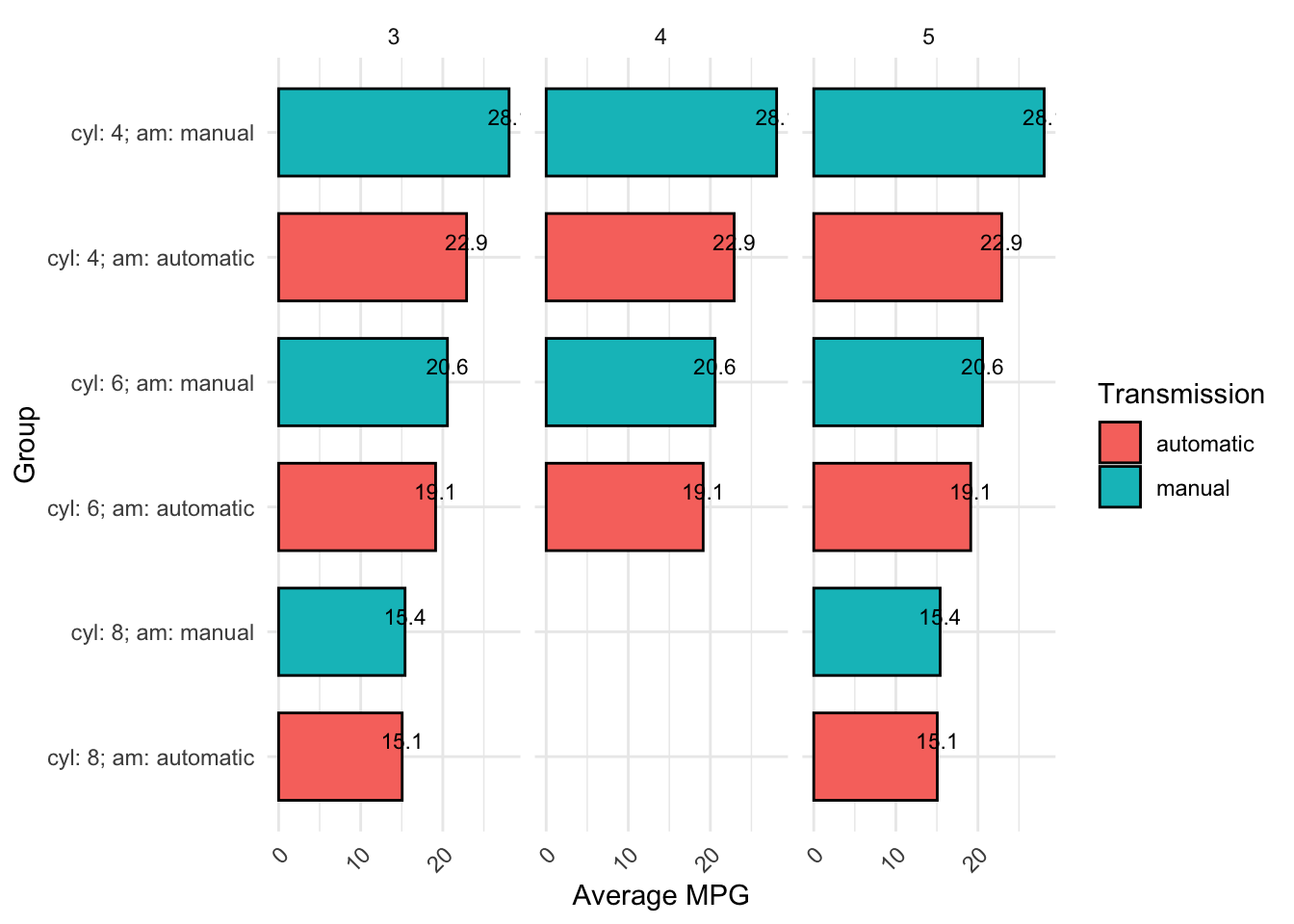

General guidelines for how to style code are laid out in ‘style guides’, such as the Tidyverse Style Guide. These are conventions rather than strict rules.

More importantly, there are R packages that will re-style your code to be compliant with the Tidyverse Style Guide. They don’t work perfectly if your code starts out as particularly poorly formatted, but they help.

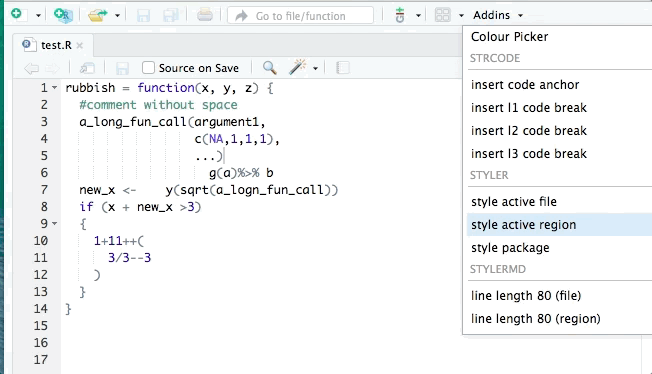
Install the {styler} R package:

install.packages("styler")
library(styler)

You can then restyle any code you’ve written by highlighting the code (click+drag) and clicking “Addins”>“STYLER”>“Style selection”. Or style the whole file with “Style active file”.

2.10 Exercises

2.10.1 Fix style / indentation / white space

Edit your local copy of this .qmd file to make the following changes. If you’re reading this as an eBook on the website, create a new .R file in RStudio on your computer (‘File>New File>R script’). Copy and paste the code below into that file.

Restyle the code with the Styler Addin.

You can undo this with Ctrl + z (Windows) or Cmd + z (Mac) if you want to see it before/after again.

library(styler)

library(dplyr)
library(ggplot2)
library(stringr)

mtcars %>% mutate(am=ifelse(am==1,
"manual","automatic"),gear=factor(
  gear
))%>%
group_by(
  cyl,am)%>%
summarise(avg_mpg=mean(mpg,na.rm=TRUE),
                       med_hp=median(hp),
                       count=n(),
                       .groups="drop"
                       )%>%
filter(avg_mpg>18|med_hp>100)%>%
mutate(flag=ifelse(avg_mpg>20&med_hp>110,TRUE,
                   FALSE),hp_per_cyl=med_hp/cyl)%>%arrange(desc(avg_mpg))%>%
left_join(
  mtcars%>%count(cyl, gear),by="cyl"  )%>%
mutate(label=str_c("cyl: ",cyl,"; am: ",am))%>%
ggplot(aes(x=reorder(
  label,
  avg_mpg
),y=avg_mpg,fill=
am))+geom_col(width  =   0.7,
              color  =   "black")+geom_text( aes( label = round(avg_mpg,1)),vjust = -0.5,size = 3)+
facet_wrap(~gear,scales="free_x")+theme_minimal(
)+theme(
axis.text.x=element_text(angle=45,hjust=1)
)+labs(
x="Group",y="Average MPG")+
guides(fill=guide_legend(title="Transmission"))+coord_flip()